Forest plot creation with ggcognigen

The creation of forest plots with ggcognigen is supported by 3 functions:

make_gmr_data: to calculate the geometric means (GM) and geometric mean ratios (GMR) of selected variables for a select list of covariates;
make_forestplot: to create forest plots based upon a data object that is typically returned by the previous function; and
make_gmr_table: to create corresponding report-ready tables in HTML, Microsoft Word, or PharmTeX-compliant format.

The make_gmr_data and make_forest_plot functions accept both standard and non-standard evaluation notations. Click here to see an example.

`make_gmr_data`

The data to be processed by make_gmr_data must meet the following expectations:

The data object must a single data.frame object.
The data in this data.frame object must be provided in wide format.
It must contain a variable that uniquely identify individuals.
It must contain one record per individual and, if requested, per stratification variable. In any cases, make_gmr_data internally filters the provided data.frame to the first record per individual and, if requested, per stratification variable.
The variables for which the GMs and GMRs are calculated must be continuous variables.
The covariates defining the groups according to which the GMs and GMRs are calculated must be factor variables.

The creation of such data objects is out of the scope of this vignette.

The operation of the make_gmr_data is explained in the examples shown below, starting from a basic case and finishing with the use of advanced settings. All examples rely on a dataset called expo which is distributed within the ggcognigen package. The expo dataset provides 3 steady-state exposures (AUCSS, CMAXSS, and CMINSS) that were predicted in a small population of individuals at 3 different dose levels (25, 50, and 100 mg), using a 1-compartment model with dose-dependent absorption. The dataset also includes the individual values of pharmacokinetic parameters (CL, V, KA, and F1) and several covariate values.

glimpse(expo)
#> Rows: 2,436
#> Columns: 17
#> $ ID     <int> 1, 2, 3, 4, 5, 6, 7, 8, 9, 10, 11, 12, 13, 14, 15, 16, 17, 18, …
#> $ DOSE   <fct> 25 mg, 25 mg, 25 mg, 25 mg, 25 mg, 25 mg, 25 mg, 25 mg, 25 mg, …
#> $ AGE    <fct> "[18,45)", "[65,90]", "[45,65)", "[18,45)", "[18,45)", "[18,45)…
#> $ WTKG   <fct> "[70.2,80)", "[89.1,100)", "[36,70.2)", "[80,89.1)", "[70.2,80)…
#> $ BMI    <fct> "[14.1,25)", "[30,40)", "[25,30)", "[30,40)", "[30,40)", "[14.1…
#> $ SEXF   <fct> Male, Female, Male, Female, Male, Female, Male, Female, Male, M…
#> $ RFCAT  <fct> Severe Impairment, Mild Impairment, Moderate Impairment, Severe…
#> $ CPCAT  <fct> Normal, Severe Impairment, Normal, Severe Impairment, Normal, M…
#> $ HFM    <fct> High fat meal, Fasted, High fat meal, Fasted, Fasted, High fat …
#> $ CL     <dbl> 12.0860, 18.9160, 19.1000, 14.2270, 11.2520, 9.3767, 8.0459, 11…
#> $ V      <dbl> 131.130, 233.300, 116.880, 237.340, 117.420, 94.863, 132.580, 2…
#> $ KA     <dbl> 0.34605, 1.10200, 0.32781, 1.03850, 0.68898, 0.97022, 0.99181, …
#> $ F1     <dbl> 0.19111, 0.30985, 0.28215, 0.32590, 0.35001, 0.23855, 0.29454, …
#> $ AUCSS  <dbl> 395.31, 409.51, 369.31, 572.68, 777.66, 636.02, 915.19, 746.19,…
#> $ TMAXSS <dbl> 4.7552, 2.4050, 4.1152, 2.6379, 3.1476, 2.5088, 2.7155, 4.2910,…
#> $ CMAXSS <dbl> 26.396, 31.874, 31.427, 38.424, 61.260, 54.106, 61.414, 43.756,…
#> $ CMINSS <dbl> 6.0931, 5.9732, 2.3850, 11.3320, 9.6471, 7.2002, 17.9770, 17.24…

Case 1: Basic use

The following example illustrates the simplest use case for make_gmr_data in which GMs and GMRs are calculated for a single exposure variable without data stratification and using default settings. By default, a 90% confidence interval is calculated for each GM and GMR. A subset of the data corresponding to the exposures obtained at 25 mg is used.

Note that, by default, the function prints information to the console while it executes. In case the call exits prematurely, this information should help the users identify which part of the data is not compatible with make_gmr_data expectations.

expo25 <- expo %>% filter(DOSE == '25 mg')
gmr25_aucss <- make_gmr_data(
  data = expo25,
  x_var = 'AUCSS',
  id_var = 'ID',
  covariates = c('AGE', 'WTKG', 'BMI', 'SEXF', 'RFCAT', 'CPCAT', 'HFM')
)
#> Data file contains 812 rows and 17 columns
#> 
#> Processing AUCSS
#> 
#> Processing AGE - Frequency table
#> 
#> [18,45) [45,65) [65,90] 
#>     404     303     105
#> ... processing group: [18,45)
#> ... processing group: [45,65)
#> ... processing group: [65,90]
#> 
#> Processing WTKG - Frequency table
#> 
#>  [36,70.2)  [70.2,80)  [80,89.1) [89.1,100)  [100,175] 
#>        162        153        172        161        164
#> ... processing group: [36,70.2)
#> ... processing group: [70.2,80)
#> ... processing group: [80,89.1)
#> ... processing group: [89.1,100)
#> ... processing group: [100,175]
#> 
#> Processing BMI - Frequency table
#> 
#> [14.1,25)   [25,30)   [30,40) [40,57.9] 
#>       159       198       400        55
#> ... processing group: [14.1,25)
#> ... processing group: [25,30)
#> ... processing group: [30,40)
#> ... processing group: [40,57.9]
#> 
#> Processing SEXF - Frequency table
#> 
#>   Male Female 
#>    375    437
#> ... processing group: Male
#> ... processing group: Female
#> 
#> Processing RFCAT - Frequency table
#> 
#>              Normal     Mild Impairment Moderate Impairment   Severe Impairment 
#>                 294                 237                 165                 116
#> ... processing group: Normal
#> ... processing group: Mild Impairment
#> ... processing group: Moderate Impairment
#> ... processing group: Severe Impairment
#> 
#> Processing CPCAT - Frequency table
#> 
#>              Normal     Mild Impairment Moderate Impairment   Severe Impairment 
#>                 292                 235                 161                 124
#> ... processing group: Normal
#> ... processing group: Mild Impairment
#> ... processing group: Moderate Impairment
#> ... processing group: Severe Impairment
#> 
#> Processing HFM - Frequency table
#> 
#>        Fasted High fat meal 
#>           557           255
#> ... processing group: Fasted
#> ... processing group: High fat meal

make_gmr_data returns a data.frame with one row per variable provided in the covariates argument and per level in these variables. The variables in this data.frame are:

x_var: the variable(s) defined in the x_var argument;
y_var: one of the variables defined in the covariates argument;
y_label: the labels associated with each variable defined in the covariates argument. It could be either the name of the variables or their ‘label’ attributes if they are defined in the input data; Alternatively, it could be one of the user-provided labels (see Case 4);
by: one of the level of the variable defined in the optional by argument (see Case 3);
value: one of the level of the covariates variables;
n: the number of individuals included in this particular level of y_var and by; records with missing value of x_var are excluded);
reference: a logical variable defining whether this particular level of y_var is the reference for the calculation of GMRs. By default, the first level of the factor is assumed to be the reference level. Alternatively, users can defines the reference levels (see Case 4);
gm: the GM value for this particular level of y_var and by;
gm_lo: the lower limit of the GM confidence interval;
gm_hi: the upper limit of the GM confidence interval;
gm_label: the GM label; structured as X1 [X2, X3], where X1 is gm}, X2 is gm_lo, X3 is gm_hi. By default, X1, X2, and X3 are formatted to 3 significant digits; alternatively, users can set the number of significant digits to use (see Case 4);
gmr: the GMR value for this particular level of y_var and bywith respect to the reference level;
gmr_lo: the lower limit of the GMR confidence interval;
gmr_hi: the upper limit of the GMR confidence interval;
gmr_label: the GMR label; structured as X1 [X2, X3], where X1 is gmr, X2 is gmr_lo, X3 is gmr_hi. By default, X1, X2, and X3 are formatted to 3 significant digits;
gmr_n_label: the GMR label with n; structured as X1 [X2, X3] n = X4, where X1 is gmr, X2 is gmr_lo, X3 is gmr_hi, X4 is n. By default, X1, X2, and X3 are formatted to 3 significant digits. This label also includes a dynamically set number of tab characters to vertically align the display of the n’s in the forest plot.

y_var, y_label, and value are coerced to factors to facilitate plotting using make_forestplot.

glimpse(gmr25_aucss)
#> Rows: 24
#> Columns: 15
#> $ x_var       <chr> "AUCSS", "AUCSS", "AUCSS", "AUCSS", "AUCSS", "AUCSS", "AUC…
#> $ y_var       <fct> AGE, AGE, AGE, WTKG, WTKG, WTKG, WTKG, WTKG, BMI, BMI, BMI…
#> $ y_label     <fct> Age (y), Age (y), Age (y), Body weight (kg), Body weight (…
#> $ value       <fct> "[18,45)", "[45,65)", "[65,90]", "[36,70.2)", "[70.2,80)",…
#> $ n           <int> 404, 303, 105, 162, 153, 172, 161, 164, 159, 198, 400, 55,…
#> $ reference   <lgl> TRUE, FALSE, FALSE, TRUE, FALSE, FALSE, FALSE, FALSE, TRUE…
#> $ gm          <dbl> 575.9795, 567.9549, 585.6130, 721.3997, 581.2538, 595.3270…
#> $ gm_lo       <dbl> 285.1323, 261.7887, 292.5570, 354.0173, 296.1954, 323.8345…
#> $ gm_hi       <dbl> 1168.0831, 1059.6106, 1078.7000, 1327.8391, 1144.5246, 103…
#> $ gm_label    <chr> "576 [285, 1170]", "568 [262, 1060]", "586 [293, 1080]", "…
#> $ gmr         <dbl> 1.0000000, 0.9860680, 1.0167254, 1.0000000, 0.8057306, 0.8…
#> $ gmr_lo      <dbl> 1.0000000, 0.9328615, 0.9403559, 1.0000000, 0.7458953, 0.7…
#> $ gmr_hi      <dbl> 1.0000000, 1.0423091, 1.0992972, 1.0000000, 0.8703658, 0.8…
#> $ gmr_label   <chr> "1 [1, 1]", "0.986 [0.933, 1.04]", "1.02 [0.94, 1.1]", "1 …
#> $ gmr_n_label <chr> "1 [1, 1]\t\t\t\tn = 404", "0.986 [0.933, 1.04]\tn = 303",…

Case 2: Multiple exposures

GMs and GMRs can be calculated for multiple exposure variables at the same call. In the example below, the silent argument is set to TRUE to suppress the display of information during execution.

gmr25_all <- make_gmr_data(
  data = expo25,
  x_var = c('AUCSS', 'CMAXSS', 'CMINSS'),
  id_var = 'ID',
  covariates = c('AGE', 'WTKG', 'BMI', 'SEXF', 'RFCAT', 'CPCAT', 'HFM'),
  silent = TRUE
)
glimpse(gmr25_all)
#> Rows: 72
#> Columns: 15
#> $ x_var       <chr> "AUCSS", "AUCSS", "AUCSS", "AUCSS", "AUCSS", "AUCSS", "AUC…
#> $ y_var       <fct> AGE, AGE, AGE, WTKG, WTKG, WTKG, WTKG, WTKG, BMI, BMI, BMI…
#> $ y_label     <fct> Age (y), Age (y), Age (y), Body weight (kg), Body weight (…
#> $ value       <fct> "[18,45)", "[45,65)", "[65,90]", "[36,70.2)", "[70.2,80)",…
#> $ n           <int> 404, 303, 105, 162, 153, 172, 161, 164, 159, 198, 400, 55,…
#> $ reference   <lgl> TRUE, FALSE, FALSE, TRUE, FALSE, FALSE, FALSE, FALSE, TRUE…
#> $ gm          <dbl> 575.97951, 567.95494, 585.61302, 721.39966, 581.25377, 595…
#> $ gm_lo       <dbl> 285.13228, 261.78865, 292.55695, 354.01730, 296.19541, 323…
#> $ gm_hi       <dbl> 1168.08314, 1059.61063, 1078.70000, 1327.83907, 1144.52458…
#> $ gm_label    <chr> "576 [285, 1170]", "568 [262, 1060]", "586 [293, 1080]", "…
#> $ gmr         <dbl> 1.0000000, 0.9860680, 1.0167254, 1.0000000, 0.8057306, 0.8…
#> $ gmr_lo      <dbl> 1.0000000, 0.9328615, 0.9403559, 1.0000000, 0.7458953, 0.7…
#> $ gmr_hi      <dbl> 1.0000000, 1.0423091, 1.0992972, 1.0000000, 0.8703658, 0.8…
#> $ gmr_label   <chr> "1 [1, 1]", "0.986 [0.933, 1.04]", "1.02 [0.94, 1.1]", "1 …
#> $ gmr_n_label <chr> "1 [1, 1]\t\t\t\tn = 404", "0.986 [0.933, 1.04]\tn = 303",…
unique(gmr25_all$x_var)
#> [1] "AUCSS"  "CMAXSS" "CMINSS"

Case 3: Stratification

GMs and GMRs can be calculated using stratification if necessary. A single stratification variable can be set in the by argument. In the example below, the whole expo data.frame is used and the calculation are stratification by DOSE.

gmr_all <- make_gmr_data(
  data = expo,
  x_var = c('AUCSS', 'CMAXSS', 'CMINSS'),
  id_var = 'ID',
  by = 'DOSE',
  covariates = c('AGE', 'WTKG', 'BMI', 'SEXF', 'RFCAT', 'CPCAT', 'HFM'),
  silent = TRUE
)
glimpse(gmr_all)
#> Rows: 216
#> Columns: 16
#> $ x_var       <chr> "AUCSS", "AUCSS", "AUCSS", "AUCSS", "AUCSS", "AUCSS", "AUC…
#> $ y_var       <fct> AGE, AGE, AGE, AGE, AGE, AGE, AGE, AGE, AGE, WTKG, WTKG, W…
#> $ y_label     <fct> Age (y), Age (y), Age (y), Age (y), Age (y), Age (y), Age …
#> $ by          <fct> 25 mg, 25 mg, 25 mg, 50 mg, 50 mg, 50 mg, 100 mg, 100 mg, …
#> $ value       <fct> "[18,45)", "[45,65)", "[65,90]", "[18,45)", "[45,65)", "[6…
#> $ n           <int> 404, 303, 105, 404, 303, 105, 404, 303, 105, 162, 153, 172…
#> $ reference   <lgl> TRUE, FALSE, FALSE, TRUE, FALSE, FALSE, TRUE, FALSE, FALSE…
#> $ gm          <dbl> 575.9795, 567.9549, 585.6130, 1722.9866, 1699.9180, 1750.4…
#> $ gm_lo       <dbl> 285.1323, 261.7887, 292.5570, 881.3175, 797.9824, 904.2484…
#> $ gm_hi       <dbl> 1168.0831, 1059.6106, 1078.7000, 3442.7852, 3123.0124, 317…
#> $ gm_label    <chr> "576 [285, 1170]", "568 [262, 1060]", "586 [293, 1080]", "…
#> $ gmr         <dbl> 1.0000000, 0.9860680, 1.0167254, 1.0000000, 0.9866113, 1.0…
#> $ gmr_lo      <dbl> 1.0000000, 0.9328615, 0.9403559, 1.0000000, 0.9349233, 0.9…
#> $ gmr_hi      <dbl> 1.0000000, 1.0423091, 1.0992972, 1.0000000, 1.0411569, 1.0…
#> $ gmr_label   <chr> "1 [1, 1]", "0.986 [0.933, 1.04]", "1.02 [0.94, 1.1]", "1 …
#> $ gmr_n_label <chr> "1 [1, 1]\t\t\t\tn = 404", "0.986 [0.933, 1.04]\tn = 303",…
unique(gmr_all[, c('x_var', 'by')])
#>      x_var     by
#> 1    AUCSS  25 mg
#> 4    AUCSS  50 mg
#> 7    AUCSS 100 mg
#> 110 CMAXSS  25 mg
#> 410 CMAXSS  50 mg
#> 73  CMAXSS 100 mg
#> 112 CMINSS  25 mg
#> 412 CMINSS  50 mg
#> 74  CMINSS 100 mg

Case 4: Advanced settings

This example illustrates the use of advanced settings.

First, a vector of integers are passed to the ref_levels argument: this vector provides the positions of the reference levels among the possible levels in each covariate variable; this vector must have the same length as the covariates argument.
Second, custom labels are provided of the covariates variable using the labels argument. This must be a vector of of character objects or expression objects with the same length as the covariates argument.
Third, a custom number of significant digit for the formatting of GM and GMR labels is set using the digits argument.
Last, a 95% CI is requested using the ci argument.

Note that all labels must be set as expression objects, if at least one of the label must be an expression. Also note the use of the ~ character to include spaces between label words. This is technically not necessary to define expressions, but the renderer function used in make_forestplot makes this syntax necessary.

gmr_all <- make_gmr_data(
  data = expo,
  x_var = c('AUCSS', 'CMAXSS', 'CMINSS'),
  id_var = 'ID',
  by = 'DOSE',
  covariates = c('AGE', 'WTKG', 'BMI', 'SEXF', 'RFCAT', 'CPCAT', 'HFM'),
  ref_levels = c(2, 3, 2, 1, 1, 1, 1),
  labels = c(
    expression('Age'~'(y)'),
    expression('Body'~'Weight'~'(kg)'),
    expression('Body'~'Mass'~'Index'~'(kg/'*m^2*')'),
    expression('Sex'),
    expression('Renal'~'Function'),
    expression('Hepatic'~'Function'~'(Child-Pugh)'),
    expression('Meal'~'Status')
  ),
  digits = 4,
  ci = 0.95,
  silent = TRUE
)
glimpse(gmr_all)
#> Rows: 216
#> Columns: 16
#> $ x_var       <chr> "AUCSS", "AUCSS", "AUCSS", "AUCSS", "AUCSS", "AUCSS", "AUC…
#> $ y_var       <fct> AGE, AGE, AGE, AGE, AGE, AGE, AGE, AGE, AGE, WTKG, WTKG, W…
#> $ y_label     <fct> "Age" ~ "(y)", "Age" ~ "(y)", "Age" ~ "(y)", "Age" ~ "(y)"…
#> $ by          <fct> 25 mg, 25 mg, 25 mg, 50 mg, 50 mg, 50 mg, 100 mg, 100 mg, …
#> $ value       <fct> "[45,65)", "[18,45)", "[65,90]", "[45,65)", "[18,45)", "[6…
#> $ n           <int> 303, 404, 105, 303, 404, 105, 303, 404, 105, 172, 162, 153…
#> $ reference   <lgl> TRUE, FALSE, FALSE, TRUE, FALSE, FALSE, TRUE, FALSE, FALSE…
#> $ gm          <dbl> 567.9549, 575.9795, 585.6130, 1699.9180, 1722.9866, 1750.4…
#> $ gm_lo       <dbl> 261.7887, 285.1323, 292.5570, 797.9824, 881.3175, 904.2484…
#> $ gm_hi       <dbl> 1059.6106, 1168.0831, 1078.7000, 3123.0124, 3442.7852, 317…
#> $ gm_label    <chr> "568 [261.8, 1060]", "576 [285.1, 1168]", "585.6 [292.6, 1…
#> $ gmr         <dbl> 1.0000000, 1.0141289, 1.0310906, 1.0000000, 1.0135704, 1.0…
#> $ gmr_lo      <dbl> 1.0000000, 0.9492420, 0.9363440, 1.0000000, 0.9505949, 0.9…
#> $ gmr_hi      <dbl> 1.0000000, 1.0834512, 1.1354245, 1.0000000, 1.0807179, 1.1…
#> $ gmr_label   <chr> "1 [1, 1]", "1.014 [0.9492, 1.083]", "1.031 [0.9363, 1.135…
#> $ gmr_n_label <chr> "1 [1, 1]\t\t\t\t\tn = 303", "1.014 [0.9492, 1.083]\t\tn =…
unique(gmr_all[, c('x_var', 'by')])
#>      x_var     by
#> 1    AUCSS  25 mg
#> 4    AUCSS  50 mg
#> 7    AUCSS 100 mg
#> 110 CMAXSS  25 mg
#> 410 CMAXSS  50 mg
#> 73  CMAXSS 100 mg
#> 112 CMINSS  25 mg
#> 412 CMINSS  50 mg
#> 74  CMINSS 100 mg

Additional settings

The paired argument can be set to TRUE if the values of the x_var variables were observed in the same individuals in all levels of each covariates. In this case, the calculation of the GMR CIs is based upon a paired t-test rather than an unpaired t-test. Study designs in which individuals are their own control could provide data amenable to the use of the paired argument.

The var.equal argument cane be set to FALSE if equal variance between the test and reference groups should NOT be assumed during the t-test.

The sep argument can be set to an alternative character, in the unforeseen case where tab characters between the CI’s and n’s are not desirable in the GM and GMR labels.

`make_forestplot`

Although the make_forestplot function ultimately returns a ggplot object, it does not rely upon the classic layer-based syntax of ggplot2. Users must call it once per plot and provide the appropriate arguments defining the properties of the plot. Nevertheless, the output of make_forestplot can be modified by standard ggplot2 functions, since it is a ggplot object.

The use and meaning of the different arguments of make_forestplot are illustrated in the examples below. Note that the code sections are hidden by default. Click on the Show / Hide button on the upper right side of each plot to display or hide the corresponding R code sections.

Basic design

In the example below, the gmr25_aucss object is re-created using custom reference levels and labels. In the call to make_forestplot:

The x, xmin, and xmax arguments are set to the variables storing the GMRs and the associated lower and upper limits of CI in the data object;
The y variable is set to the variable storing the different covariate levels;
The facet variable is set to the variable storing the covariate labels;
The label variable is set to the variable storing the GMR labels (in this case GMR + n labels);
The vline_primary and vline_secondary arguments define some primary and secondary values of references;
The fatten argument control the thickness of symbols and lines on the plots;
The small_font argument is passed down to a call to theme_cognigen_grid and controls whether a smaller font size is used for text displays;
The xlb, ylb (not used below), and title are character or expression objects defining axis and plot titles.

gmr25_aucss <- make_gmr_data(
  data = expo25,
  x_var = 'AUCSS',
  id_var = 'ID',
  covariates = c('AGE', 'WTKG', 'BMI', 'SEXF', 'RFCAT', 'CPCAT', 'HFM'),
  ref_levels = c(2, 3, 2, 1, 1, 1, 1),
  labels = c(
    expression('Age'~'(y)'),
    expression('Body'~'Weight'~'(kg)'),
    expression('Body'~'Mass'~'Index'~'(kg/'*m^2*')'),
    expression('Sex'),
    expression('Renal'~'Function'),
    expression('Hepatic'~'Function'~'(Child-Pugh)'),
    expression('Meal'~'Status')
  ),
  silent = TRUE
)
p1 <- make_forestplot(
  data = gmr25_aucss,
  y = 'value', x = 'gmr', xmin = 'gmr_lo', xmax = 'gmr_hi',
  label = 'gmr_n_label',
  facet = 'y_label',
  vline_primary = 1,
  vline_secondary = c(0.8, 1.25),
  xlb = 'Geometric Mean Ratio [90% confidence interval]',
  title = expression(AUC[ss*','~0 ~'-'~24~h]~'(nmol' %*% 'h/L)'),
  fatten = 2,
  small_font = TRUE
)
p1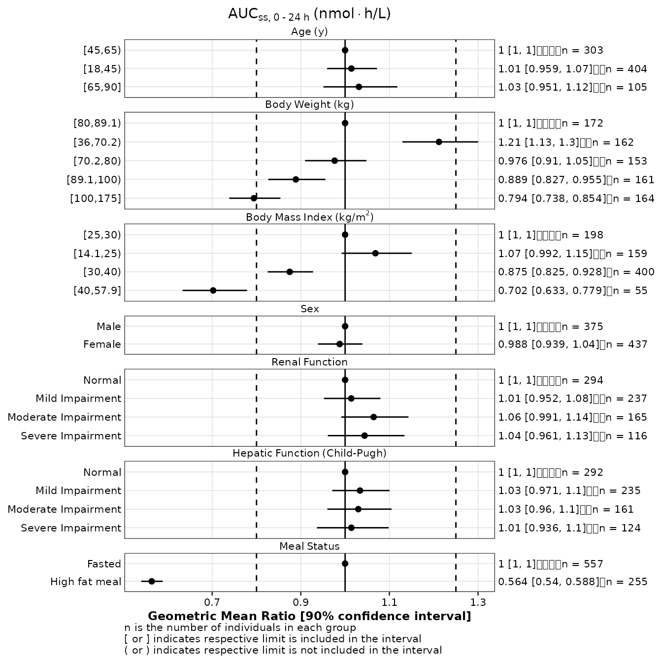

Note that, although the alignment of the n counts appears incorrect on the right of the plot shown above, it will be correct once the plot in save to a png file.

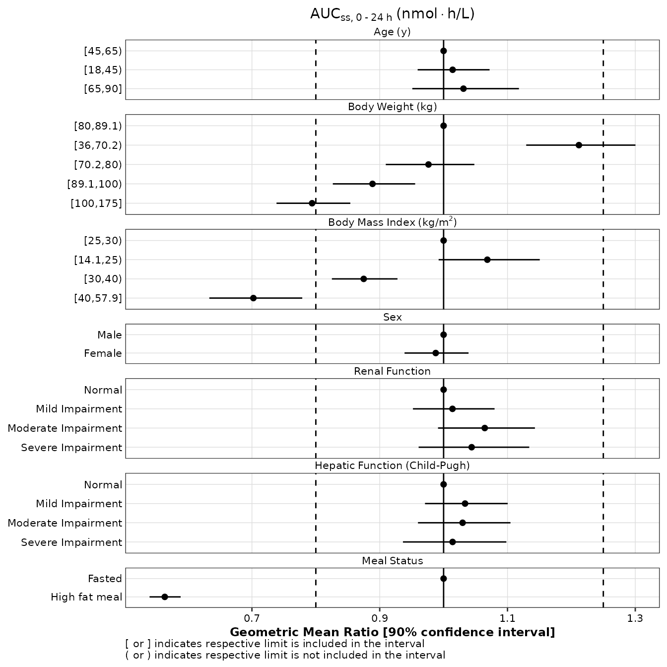
When GMR labels are not desired, the label argument can be set to NULL or simply not included in the call.

make_forestplot(
  data = gmr25_aucss,
  y = 'value', x = 'gmr', xmin = 'gmr_lo', xmax = 'gmr_hi',
  label = NULL,
  facet = 'y_label',
  vline_primary = 1,
  vline_secondary = c(0.8, 1.25),
  xlb = 'Geometric Mean Ratio [90% confidence interval]',
  title = expression(AUC[ss*','~0 ~'-'~24~h]~'(nmol' %*% 'h/L)'),
  fatten = 2,
  small_font = TRUE
)

Non-standard evaluation

Below, tidyverse-style syntax and unquoted variables are used to reproduce the same forest plot as above.

gmr25_aucss <- expo25 %>%
  make_gmr_data(
    x_var = AUCSS,
    id_var = ID,
    covariates = c(AGE, WTKG, BMI, SEXF, RFCAT, CPCAT, HFM),
    ref_levels = c(2, 3, 2, 1, 1, 1, 1),
    labels = c(
      expression('Age'~'(y)'),
      expression('Body'~'Weight'~'(kg)'),
      expression('Body'~'Mass'~'Index'~'(kg/'*m^2*')'),
      expression('Sex'),
      expression('Renal'~'Function'),
      expression('Hepatic'~'Function'~'(Child-Pugh)'),
      expression('Meal'~'Status')
    ),
    silent = TRUE
  )
p1 <- make_forestplot(
  data = gmr25_aucss,
  y = value, x = gmr, xmin = gmr_lo, xmax = gmr_hi,
  label = NULL,
  facet = y_label,
  vline_primary = 1,
  vline_secondary = c(0.8, 1.25),
  xlb = 'Geometric Mean Ratio [90% confidence interval]',
  title = expression(AUC[ss*','~0 ~'-'~24~h]~'(nmol' %*% 'h/L)'),
  fatten = 2,
  small_font = TRUE
)
p1

Defining what `n` is

By default, forest plots created with make_forestplot identify a data point as an individual (see footnote of the 1st plot in the previous section). You can use the n_label argument to change this default if necessary:


make_forestplot(
  data = gmr25_aucss,
  y = 'value', x = 'gmr', xmin = 'gmr_lo', xmax = 'gmr_hi',
  label = 'gmr_n_label',
  facet = 'y_label',
  vline_primary = 1,
  vline_secondary = c(0.8, 1.25),
  xlb = 'Geometric Mean Ratio [90% confidence interval]',
  title = expression(AUC[ss*','~0 ~'-'~24~h]~'(nmol' %*% 'h/L)'),
  n_label = 'patient',
  fatten = 2,
  small_font = TRUE
)

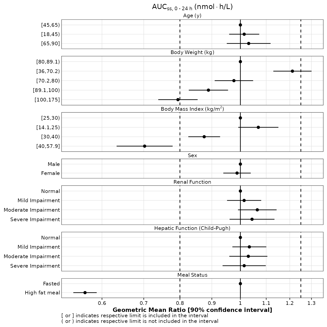
Logarithmic scale for x-axis

The scale of the X-axis can be changed to logarithmic scale as follows (see stratification section below if log scale and stratification are simultaneously needed):

p1 + scale_x_continuous(
  trans = 'log10',
  breaks = c(0.6, 0.7, 0.8, 0.9, 1, 1.1, 1.2, 1.3, 1.4),
  labels = format_continuous_cognigen
)

Highlight reference group

The reference group can be displayed with a unique symbol when the reference argument is set to the logical variable storing with information in data

make_forestplot(
  data = gmr25_aucss,
  y = 'value', x = 'gmr', xmin = 'gmr_lo', xmax = 'gmr_hi',
  label = 'gmr_n_label',
  facet = 'y_label',
  reference = 'reference',
  vline_primary = 1,
  vline_secondary = c(0.8, 1.25),
  xlb = 'Geometric Mean Ratio [90% confidence interval]',
  title = expression(AUC[ss*','~0 ~'-'~24~h]~'(nmol' %*% 'h/L)'),
  fatten = 2,
  small_font = TRUE
)

Reordering covariate groups

As mentioned above, the y_var, y_label, and value variables in the output of make_gmr_data are coerced to factors to facilitate plotting using make_forestplot. Within a series of covariate levels, the reference level is always listed first in the output data.frame. This may not always be desirable.

Users can modify the reorder the levels of the value factor to modify the

gmr25_aucss <- gmr25_aucss %>% 
  mutate(
    value_mod = factor(value, levels(value)[c(2, 1, 3, 5, 6, 4, 7, 8, 10, 9, 11:20)])
  )
levels(gmr25_aucss$value)
#>  [1] "[45,65)"             "[18,45)"             "[65,90]"            
#>  [4] "[80,89.1)"           "[36,70.2)"           "[70.2,80)"          
#>  [7] "[89.1,100)"          "[100,175]"           "[25,30)"            
#> [10] "[14.1,25)"           "[30,40)"             "[40,57.9]"          
#> [13] "Male"                "Female"              "Normal"             
#> [16] "Mild Impairment"     "Moderate Impairment" "Severe Impairment"  
#> [19] "Fasted"              "High fat meal"
levels(gmr25_aucss$value_mod)
#>  [1] "[18,45)"             "[45,65)"             "[65,90]"            
#>  [4] "[36,70.2)"           "[70.2,80)"           "[80,89.1)"          
#>  [7] "[89.1,100)"          "[100,175]"           "[14.1,25)"          
#> [10] "[25,30)"             "[30,40)"             "[40,57.9]"          
#> [13] "Male"                "Female"              "Normal"             
#> [16] "Mild Impairment"     "Moderate Impairment" "Severe Impairment"  
#> [19] "Fasted"              "High fat meal"

make_forestplot(
  data = gmr25_aucss,
  y = 'value_mod', x = 'gmr', xmin = 'gmr_lo', xmax = 'gmr_hi',
  label = 'gmr_n_label',
  facet = 'y_label',
  reference = 'reference',
  vline_primary = 1,
  vline_secondary = c(0.8, 1.25),
  xlb = 'Geometric Mean Ratio [90% confidence interval]',
  title = expression(AUC[ss*','~0 ~'-'~24~h]~'(nmol' %*% 'h/L)'),
  fatten = 2,
  small_font = TRUE
)

Coloring

If the color argument is added to the call to make_forestplot, the data shown in the forest plot can be colored according to the value of the defined variable. This requires that the data object passed to the function include a relevant value, which typically has to be created after execution of the make_gmr_data function. For instance, it may be useful to color the GMR based upon their location with respect to the vline_secondary boundaries as shown below.

gmr25_aucss <- gmr25_aucss %>% 
  mutate(
    group = factor(
      ifelse(
        is.na(gmr),
        1,
        ifelse(
          gmr >= 0.8 & gmr <= 1.25,
          ifelse( gmr_lo < 0.8 | gmr_hi > 1.25, 2, 1),
          ifelse( gmr_hi < 0.8 | gmr_lo > 1.25, 4, 3)
        )
      ),
      labels = c('CI inside limits', 'CI partially outside limits', 'GMR outside limits', 'CI fully ouside limits')
    )
  )

make_forestplot(
  data = gmr25_aucss,
  y = 'value_mod', x = 'gmr', xmin = 'gmr_lo', xmax = 'gmr_hi',
  label = 'gmr_n_label',
  color = 'group',
  facet = 'y_label',
  reference = 'reference',
  vline_primary = 1,
  vline_secondary = c(0.8, 1.25),
  xlb = 'Geometric Mean Ratio [90% confidence interval]',
  title = expression(AUC[ss*','~0 ~'-'~24~h]~'(nmol' %*% 'h/L)'),
  fatten = 2,
  small_font = TRUE
) + 
  scale_color_manual(values = c('#008000', '#0000FF', '#FFA000', '#FF0000')) +
  labs(color = '')  # to remove the legend title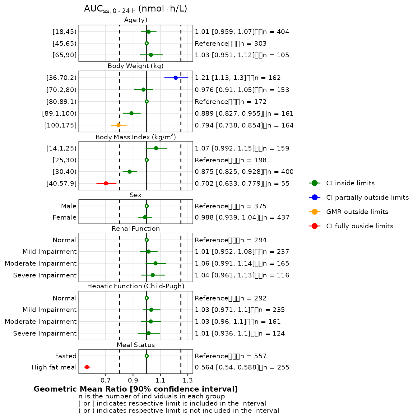

Stratification

If the data object passed to make_forestplot contains multiple records per combinations of the y and color variables, the function automatically detects that the data must be stratified and colored in the forest plot.

gmr_all <- make_gmr_data(
  data = expo,
  x_var = c('AUCSS', 'CMAXSS', 'CMINSS'),
  id_var = 'ID',
  by = 'DOSE',
  covariates = c('AGE', 'WTKG', 'BMI', 'SEXF', 'RFCAT', 'CPCAT', 'HFM'),
  ref_levels = c(2, 3, 2, 1, 1, 1, 1),
  labels = c(
    expression('Age'~'(y)'),
    expression('Body'~'Weight'~'(kg)'),
    expression('Body'~'Mass'~'Index'~'(kg/'*m^2*')'),
    expression('Sex'),
    expression('Renal'~'Function'),
    expression('Hepatic'~'Function'~'(Child-Pugh)'),
    expression('Meal'~'Status')
  ),
  silent = TRUE
)
p2 <- make_forestplot(
  data = subset(gmr_all, x_var == 'AUCSS'),
  y = 'value', x = 'gmr', xmin = 'gmr_lo', xmax = 'gmr_hi',
  label = 'gmr_n_label',
  color = 'by',
  facet = 'y_label',
  vline_primary = 1,
  vline_secondary = c(0.8, 1.25),
  xlb = 'Geometric Mean Ratio [90% confidence interval]',
  title = expression(AUC[ss*','~0 ~'-'~24~h]~'(nmol' %*% 'h/L)'),
  fatten = 2,
  small_font = TRUE
) +
  scale_discrete_cognigen() +
  labs(color = '')  # to remove the legend title
p2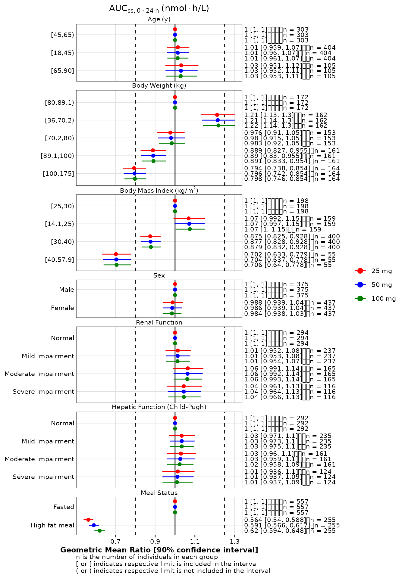

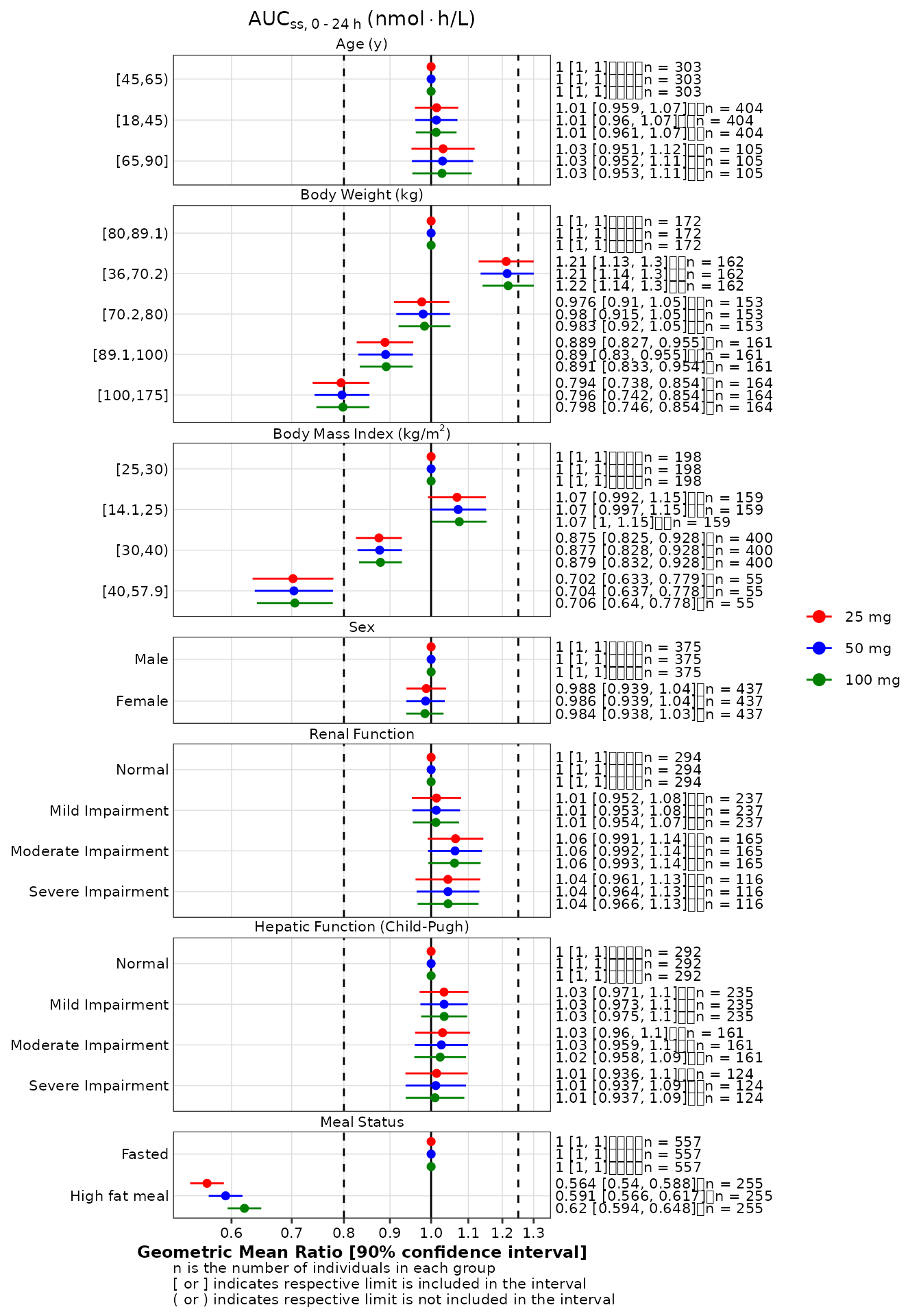
Because the implementation of stratification requires the use of facet-specific scales, the X-axis scale cannot be change globally. If a logarithmic scale is required, users must apply the approach illustrated in the example below. In brief, a scale_x_continuous function is created and applied to each panel using the ggh4x::facetted_pos_scales function. A list with as many levels as there are panels must be created.

logscale <- scale_x_continuous(
  trans = 'log10',
  breaks = c(0.6, 0.7, 0.8, 0.9, 1, 1.1, 1.2, 1.3, 1.4),
)
p2 +
  ggh4x::facetted_pos_scales(
    x = list(
      # one element per panel
      logscale,
      logscale,
      logscale,
      logscale,
      logscale,
      logscale,
      logscale
    )
  )

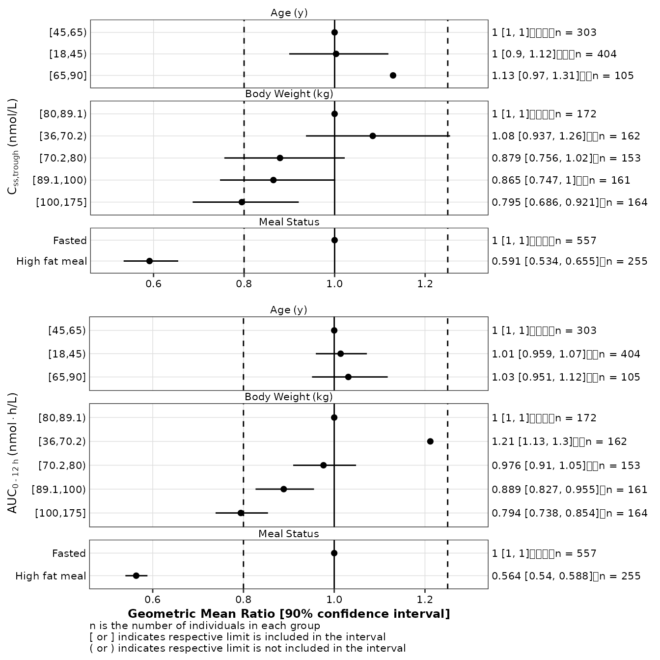
Multiple exposures

Displaying GMRs for multiple exposures on the same plots is not directly possible with make_forestplot but this design can be achieved using the following approach:

Users must create one forest plot per exposure;
All N plots must share the same X-axis limits and the same vline_primary and vline_secondary settings;
For all plots above the bottom one, the title of the X-axis and the footnote must be turned off;
The Y-axis title is used to information about the exposures associated which each individual forest plots;
An empty ggplot plot object must be created; and
A Nx2 layout must be created and the plots arranged with ggpubr::ggarrange as shown below (not that the second column of plot is necessary to circumvent a bug with ggarrange with does not properly process the secondary y-axis axis showing the GMR labels).

gmr25_all <- make_gmr_data(
  data = expo25,
  x_var = c('AUCSS', 'CMAXSS', 'CMINSS'),
  id_var = 'ID',
  covariates = c('AGE', 'WTKG', 'HFM'),
  ref_levels = c(2, 3, 1),
  labels = c(
    expression('Age'~'(y)'),
    expression('Body'~'Weight'~'(kg)'),
    expression('Meal'~'Status')
  ),
  silent = TRUE
)
p1_1 <- make_forestplot(
  data = subset(gmr25_all, x_var == 'CMINSS'),
  y = 'value', x = 'gmr', xmin = 'gmr_lo', xmax = 'gmr_hi',
  label = 'gmr_n_label',
  facet = 'y_label',
  vline_primary = 1,
  vline_secondary = c(0.8, 1.25),
  xlb = NULL,
  ylb = expression(C[ss*','*trough]~'(nmol/L)'),
  fatten = 2,
  small_font = TRUE
) +
  ggplot2::xlim( c(0.5, 1.3) ) +
  ggplot2::labs( caption = NULL )

p1_2 <- make_forestplot(
  data = subset(gmr25_all, x_var == 'AUCSS'),
  y = 'value', x = 'gmr', xmin = 'gmr_lo', xmax = 'gmr_hi',
  label = 'gmr_n_label',
  facet = 'y_label',
  vline_primary = 1,
  vline_secondary = c(0.8, 1.25),
  xlb = 'Geometric Mean Ratio [90% confidence interval]',
  ylb = expression(AUC[0 ~'-'~12~h]~'(nmol' %*% 'h/L)'),
  fatten = 2,
  small_font = TRUE
) +
  ggplot2::xlim( c(0.5, 1.3) )

p2_1 <- ggplot() + theme_void()

suppressWarnings(
  ggpubr::ggarrange(
    p1_1, p2_1, p1_2,
    nrow = 2, ncol = 2,
    widths = c(0.95, 0.05),
    heights = c(0.45, 0.55)
  )
)

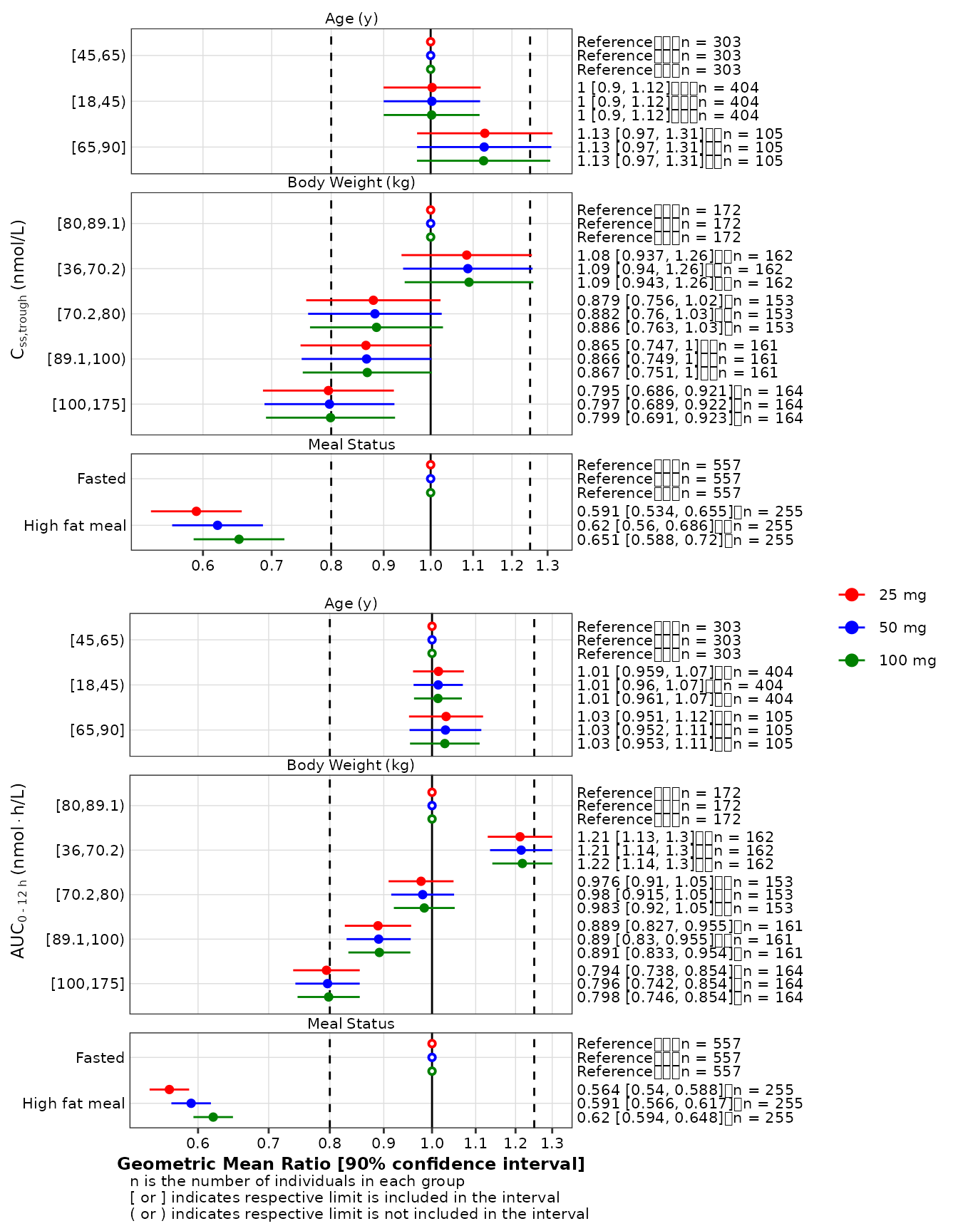
All-at-once

In this example, all possible options are use. The combination of data stratification, display of multiple exposures, and logarithmic scale requires additional tricks:

ggh4x::facetted_pos_scales must be called to apply the logarithmic scale to each forest plot;
The legend must be suppressed in each forest plot. However, it must be extracted with ggpubr::get_legend in at least 1 forest plot before being suppressed;
A nest layout must be used to vertically center the legend: in the case below, a 2x2 layout within a 1x2 layout.

gmr_all <- make_gmr_data(
  data = expo,
  x_var = c('AUCSS', 'CMAXSS', 'CMINSS'),
  id_var = 'ID',
  covariates = c('AGE', 'WTKG', 'HFM'),
  ref_levels = c(2, 3, 1),
  by = 'DOSE',
  labels = c(
    expression('Age'~'(y)'),
    expression('Body'~'Weight'~'(kg)'),
    expression('Meal'~'Status')
  ),
  silent = TRUE
)
p1_1 <- make_forestplot(
  data = subset(gmr_all, x_var == 'CMINSS'),
  y = 'value', x = 'gmr', xmin = 'gmr_lo', xmax = 'gmr_hi',
  label = 'gmr_n_label',
  facet = 'y_label',
  color = 'by',
  reference = 'reference',
  vline_primary = 1,
  vline_secondary = c(0.8, 1.25),
  xlb = NULL,
  ylb = expression(C[ss*','*trough]~'(nmol/L)'),
  fatten = 2,
  small_font = TRUE
) +
  ggh4x::facetted_pos_scales(
    x = list(
      logscale,
      logscale,
      logscale
    )
  ) +
  ggplot2::scale_color_manual(
    values = get_style_colors(cognigen_style())[-1]
  ) + 
  ggplot2::xlim( c(0.5, 1.3) ) +
  ggplot2::labs( caption = NULL ) +
  labs(color = '')

# Extract the legend before suppressing it
plegend <- ggpubr::get_legend(p1_1)
p1_1 <- p1_1 +
  theme(legend.position = 'none')

p1_2 <- make_forestplot(
  data = subset(gmr_all, x_var == 'AUCSS'),
  y = 'value', x = 'gmr', xmin = 'gmr_lo', xmax = 'gmr_hi',
  label = 'gmr_n_label',
  facet = 'y_label',
  color = 'by',
  reference = 'reference',
  vline_primary = 1,
  vline_secondary = c(0.8, 1.25),
  xlb = 'Geometric Mean Ratio [90% confidence interval]',
  ylb = expression(AUC[0 ~'-'~12~h]~'(nmol' %*% 'h/L)'),
  fatten = 2,
  small_font = TRUE
)  +
  ggh4x::facetted_pos_scales(
    x = list(
      logscale,
      logscale,
      logscale
    )
  ) +
  ggplot2::scale_color_manual(
    values = get_style_colors(cognigen_style())[-1]
  ) +
  ggplot2::xlim( c(0.5, 1.3) ) +
  theme(legend.position = 'none')

p2_1 <- ggplot() + theme_void()

suppressWarnings(
  ggpubr::ggarrange(
  ggpubr::ggarrange(
    p1_1, p2_1, p1_2, 
    nrow = 2, ncol = 2, 
    widths = c(0.95, 0.05),
    heights = c(0.475, 0.525)
  ),
  plegend,
  nrow = 1,
  ncol = 2,
  widths = c(0.85, 0.15)
)
)

Note that it is not recommended to use scale_discrete_cognigen with make_forestplot as it would override some scale settings defined with the function itself. Instead use scale_color_manual combined with get_style_colors as illustrated above.

`make_gmr_table`

make_gmr_table creates report-ready tables of GMs and GMRs data in HTML, Microsoft Word, or PharmTeX-compliant format. This is a relatively simple function which only makes a few assumptions about the data it processes. It was designed to print the output of the make_gmr_data output data.frame but typically requires that data.frame to be slightly modified beforehand. These modifications may include dropping one or more unnecessary variables and converting expression into character objects (using the expr2char utility function).

Users will be able to set the name of the output table file, request the desired format, and set custom table headers and add a list of custom abbreviations to those that are automatically included by make_gmr_table (i.e., CI and n).

make_gmr_table can creates one or more table files at a time, as illustrated below.


# Preprocessing 
gmr_table_data <- gmr_all[, c('x_var', 'y_label', 'value', 'by', 'n', 'gm_label','gmr_label')]
levels(gmr_table_data[, 'y_label']) <- expr2char(levels(gmr_table_data[, 'y_label']))

# Request html table
make_gmr_table(
  data = gmr_table_data,
  file = 'gmtable.html',
  format = 'html',
  headers = c(
    'Exposure Measure',
    'Covariate',
    'Group',
    'Dose',
    'n',
    'Geometric Mean [90% CI]',
    'Geometric Mean Ratio [90% CI]'
  ),
  abbreviations = list(
    ABC = 'Some custom variable',
    XYZ = 'Another custom variable'
  )
)

# Request Word table
make_gmr_table(
  data = gmr_table_data,
  file = 'gmtable.docx',
  format = 'word',
  title = 'Mouh',
  headers = c(
    'Exposure Measure',
    'Covariate',
    'Group',
    'n',
    'Geometric Mean [90% CI]',
    'Geometric Mean Ratio [90% CI]'
  ),
  abbreviations = list(
    ABC = 'Some custom variable',
    XYZ = 'Another custom variable'
  )
)

# Request both with one call
make_gmr_table(
  data = gmr_table_data,
  file = c('gmtable.html, gmtable.docx'),
  format = c('html', 'word'),
  title = 'Mouh',
  headers = c(
    'Exposure Measure',
    'Covariate',
    'Group',
    'n',
    'Geometric Mean [90% CI]',
    'Geometric Mean Ratio [90% CI]'
  ),
  abbreviations = list(
    ABC = 'Some custom variable',
    XYZ = 'Another custom variable'
  )
)

Sebastien Bihorel

for the Clinical Pharmacology and Pharmacometrics (CPP) business unit of Simulations Plus, Inc

`make_gmr_data`

Case 1: Basic use

Case 2: Multiple exposures

Case 3: Stratification

Case 4: Advanced settings

Additional settings

`make_forestplot`

Basic design

Non-standard evaluation

Defining what `n` is

Logarithmic scale for x-axis

Highlight reference group

Reordering covariate groups

Coloring

Stratification

Multiple exposures

All-at-once

`make_gmr_table`

Forest plot creation with ggcognigen

Sebastien Bihorel

for the Clinical Pharmacology and Pharmacometrics (CPP) business unit of Simulations Plus, Inc

make_gmr_data

Case 1: Basic use

Case 2: Multiple exposures

Case 3: Stratification

Case 4: Advanced settings

Additional settings

make_forestplot

Basic design

Non-standard evaluation

Defining what n is

Logarithmic scale for x-axis

Highlight reference group

Reordering covariate groups

Coloring

Stratification

Multiple exposures

All-at-once

make_gmr_table

`make_gmr_data`

`make_forestplot`

Defining what `n` is

`make_gmr_table`